Adaptive Control using Multiple Models
Table of Contents:
This post has been adapted from a university project to understand and simulate the findings of [1]
Preamble
The evolution of a dynamical system is mathematically modeled as differential equations. Properties of the system like position and velocity at any given moment are the State of the system. Differential equations capture how these states change and influence each other over time.
The mathematical models imply that a given system (or Plant) would follow a deterministic trajectory for a given initial state. For example, an airplane would remain at rest if it is parked on level ground. It would glide down if it is released at 1000 feet above in the air with a particular initial velocity and orientation.
But we often want to do more with systems than to let them follow their natural trajectories. And we cannot always precisely set or measure initial conditions. We want more Control.
Thus we influence some properties of the dynamical system by applying a control input. For example applying torque to the wheels of your car, or by propelling the motors of an airplane to create thrust that pushes it forward. This control input directly or indirectly alters the state of our system.
A control designer’s job is to ensure that the system follows a trajectory of our choice, which is often represented as a Reference Model; and to ensure stability of the overall system, i.e. it does not behave erratically on small deviations.
PID Controller
For simple single-order plants, an often effective strategy is to change the control input in proportion to the difference (or error) between the plant state and reference state.
The error term is often integrated over time to capture the past, and differentiated to capture the instantaneous future of the error. The three terms (Proportional, Integral, Derivative) are used together in different proportions to design a control input, resulting in a PID Controller.
The performance of simple PID controllers isn’t always good enough, and the control law is not designed to the specification of plant dynamics and parameters, but only to its output.
Especially for complex multi-order plants, a lot of information is lost if we use only the plant output to control it and not the known information about its internal dynamics.
Adaptive Control
Many times the parameters of the dynamical system are not completely known, or they are changing as the system evolves. In such scenarios, we need to adaptively change the control law itself with time.
Adaptive control primarily focuses on system identification (i.e. estimating the parameters of the system) to design the control input; and using Lyapunov analysis to ensure stability of the system.
Plant Model
Let’s start with the simple case of a multi-order linear plant. Its dynamics can be described in state-space form as:
\[\dot{x}_p(t) = A_p x_p(t) + bu(t)\]Where \(x_p\) is the n-dimensional state space vector, \(A_p\) are the parameters as a \(n \times n\) companion matrix. \(u\) is the control input, and \(b = [0, \cdots, 0, 1]^T\)
Side Note: More details on how to represent an nth order d.e. in state-space form with companion matrices is given here
\[\begin{bmatrix} \dot{x_1} \\ \dot{x_2} \\ \vdots \\ \dot{x_{n-1}} \\ \dot{x_n} \end{bmatrix} = \begin{bmatrix} 0 & 1 & 0 & \cdots & 0 \\ 0 & 0 & 1 & \cdots & 0 \\ \vdots & \vdots & \vdots & \ddots & \vdots \\ 0 & 0 & 0 & \cdots & 1 \\ -a_1 & -a_2 & -a_3 & \cdots & -a_n \end{bmatrix} \begin{bmatrix} x_1 \\ x_2 \\ \vdots \\ x_{n-1} \\ x_n \end{bmatrix} + \begin{bmatrix} 0 \\ 0 \\ \vdots \\ 0 \\ 1 \\ \end{bmatrix} u\]The last row of the companion matrix \(A_p\) is the parameter vector \(\theta_p\), which can also be represented as:
\[\theta_p = \begin{bmatrix} -a_1 \\ -a_2 \\ \vdots \\ -a_n \end{bmatrix}\]Reference Model
A reference model that this plant should track can be described via a similar set of equations:
\[\dot{x}_m(t) = A_m x_m(t) + br(t)\]Where \(x_m\) and \(A_m\) are described similarly, and \(r\) is a known reference signal.
Identification Model
Before we proceed to designing our control law, we need to estimate the plant parameters \(\theta_p\), as they are unknown to us.
To achieve that we set up an identification model as follows:
\[\dot{x}_I(t) = A_m x_I(t) + [A_I - A_m] x_p(t) + bu(t)\]Where \(A_I\) is a matrix in companion form with its last row as the plant parameter estimate \(\theta_I\). The identification error \(e_I\) is defined as:
\[e_I(t) = x_I(t) - x_p(t)\]Adaptive Law
Let \(P\) be the positive definite matrix solution to the lyapunov equation for the reference model:
\[A_m^T P + P A_m = -Q, Q = Q^T > 0\]Where our Lyapunov function candidate is defined as:
\[V = e_I^T P e_I + \bar{\theta}_I^T \bar{\theta}_I\]Theorem 1
If we define our parameter adaptive law as:
\[\dot{\theta}_I(t) = -e_I^T(t) P b x_p(t)\]we end up with a stable system under Lyapunov criteria:
\[\dot{V} = -e_I^T Q e_I \leq 0\]Control Law
Using the Lyapunov stability analysis, we can define our control input as:
\[u(t) = -k^T(t) x_p(t) + r(t)\]Where \(k(t) = \theta_I(t) - \theta_m\). From Barbalat’s lemma it follows that the tracking error \(e_c\) approaches 0 \(\lim_{t \rightarrow \infty} e_c(t) = 0\), or in other words that \(x_p\) tracks \(x_m\).
Simulation 1
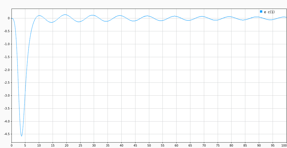
For a second order plant, with parameters \(\theta_p = [-7, -2]^T\) tracking a reference model with \(\theta_m = [-5, -6]^T\). We initialize our identification model with \(\theta_i = [-8, -4]^T\). The tracking signal is \(r(t) = 5\sin(0.2\pi t)\).
(d/l multidim_singlemodel.slx)
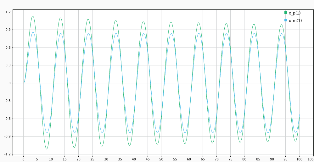
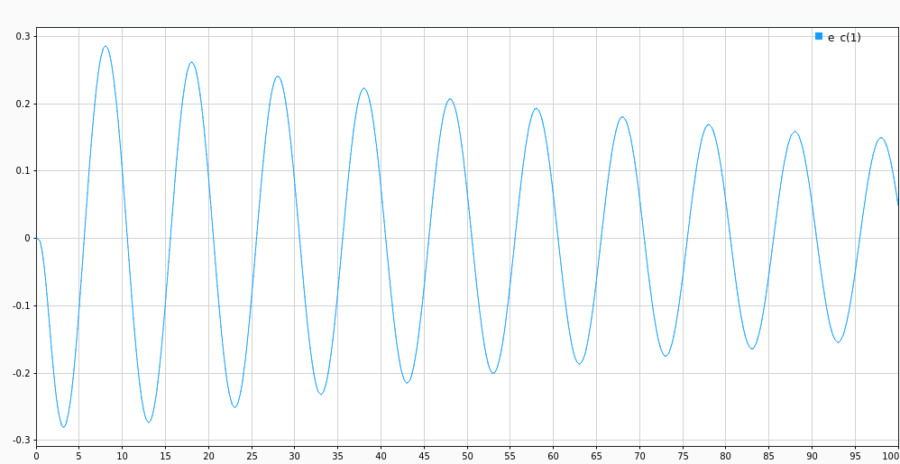
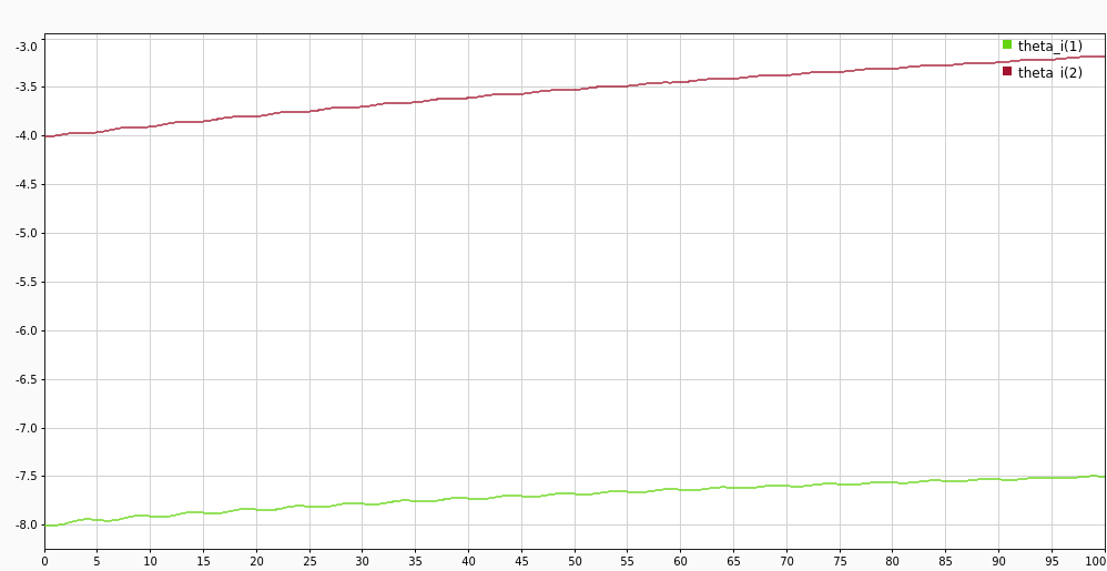
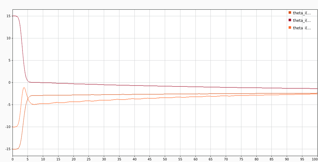
The tracking error \(e_c\) dies down slowly. This is because the parameter estimates \(\theta_i\) converge to the plant values \(\theta_p\) very slowly (as seen in the following figure).
Multiple Identification Models
Level 1
Let us use \(N = n + 1\) identification models, defined similarly as before, with same initial state as \(x_p\), but different initial values for the parameter estimate \(\theta_i\):
\[\dot{x}_i(t) = A_m x_i(t) + [A_i - A_m] x_p(t) + bu(t)\]Despite having \(N\) models, we can still only have a single control input. We achieve that by taking a convex combination of the parameter estimates as:
\[\theta_I(t) = \sum_{i=1}^N \alpha_i \theta_i(t)\]Where \(\sum_{i=1}^N \alpha_i = 1\). We can restate this in matrix-vector notation, with \(\theta_i\) as columns of \(\Theta_I\), and \(\alpha = [\alpha_1, \alpha_2, \cdots, \alpha_N]^T\):
\[\theta_I(t) = \Theta_I(t) \alpha\]Theorem 2
If \(N\) adaptive identification models are initialized as \(\theta_i(t_0)\) such that \(x_i(t_0) = x_p(t_0)\), and plant parameter vector \(\theta_p\) lies in the convex hull of \(\theta_i(t_0)\), then \(\theta_p\) continues to lie in the convex hull of \(\theta_i(t), t > t_0\).
Simulation 2
For a second order plant, with parameters \(\theta_p = [-2, 9]^T\) tracking same reference model as before \(\theta_m = [-5, -6]^T\). We initialize our identification model with \(\alpha = [0.7, 0.1, 0.2]^T\) and
\[\theta_I(t_0) = \begin{bmatrix} -15 & 15 & -10 \\ 10 & 15 & -10 \end{bmatrix}\](d/l multidim_multimodel.slx)
Tracking error \(e_c\) still dies down slowly in the later phase. Despite having multiple models, we’re still estimating only one value in the convex hull of the multiple models. And the individual parameter errors of the models are still converging slowly to the actual value.
Level 2
Level 1 leads to an equivalent performing system as before, albeit using multiple models. The key insight is to adaptively estimate \(\alpha\) itself, along with each model’s parameters.
The conclusion of theorem 2 can be restated as:
\[\theta_p(t) = \sum_{i=1}^N \alpha_i \theta_i(t), t \geq t_0\]Subtracting \(\theta_p\) from both sides:
\[\sum_{i=1}^N \alpha_i e_i(t) = 0\] \[[e_1(t), e_2(t), \cdots, e_N(t)] \alpha = E(t) \alpha = 0\]The previous equation can be simplified down using:
\[\sum_{i=1}^N \alpha_i = 1 \implies 1 - \sum_{i=1}^{N-1} \alpha_i = \alpha_N\]Substituting \(\bar{\alpha} = [\alpha_1, \alpha_2, \cdots, \alpha_{N-1}]^T\) leads to:
\[\begin{bmatrix}e_1(t) & e_2(t) & \cdots & e_N(t)\end{bmatrix} \begin{bmatrix}\bar{\alpha} \\ 1 - \sum_{i=1}^{N-1} \alpha_i\end{bmatrix} = 0\] \[\begin{bmatrix} e_1(t) - e_N(t) & e_2(t) - e_N(t) & \cdots & e_{N-1}(t) - e_N(t)\end{bmatrix} \bar{\alpha} = -e_N(t)\] \[\bar{E}(t) \bar{\alpha} = h(t)\]Estimate \(\bar{\alpha}\)
We can now use a standard estimation process for \(\bar{\alpha}\) like we did for parameters before. Let \(\hat{\bar{\alpha}}(t)\) be its estimation, then the adaptive law is given by:
\[\dot{\hat{\bar{\alpha}}}(t) = -\bar{E}^T(t) [\hat{h}(t) - h(t)]\]Theorem 3
Using analysis similar to Theorem 1, we can show that the second level of adaptation also leads to an overall stable system. And when convergence is slow in first level (i.e. large parametric errors), convergence of \(\hat{\bar{\alpha}}\) to \(\bar{\alpha}\) is rapid. (and vice versa)
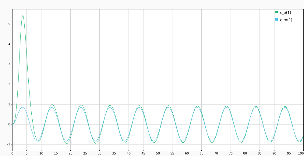
Simulation 3
For the same second order plant as in Simulation 2. That is \(\theta_p = [-7, -2]^T\), \(\theta_m = [-5, -6]^T\). This time we initialize our identification model with \(\hat{\bar{\alpha}}(t_0) = [0.7, 0.1, 0.2]^T\) estimating it on the fly along with plant parameters with
\[\theta_I(t_0) = \begin{bmatrix} -15 & 15 & -10 \\ 10 & 15 & -10 \end{bmatrix}\](d/l multidim_multimodel_lvl2.slx)
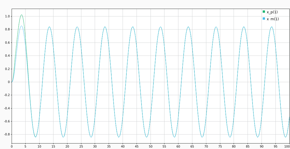
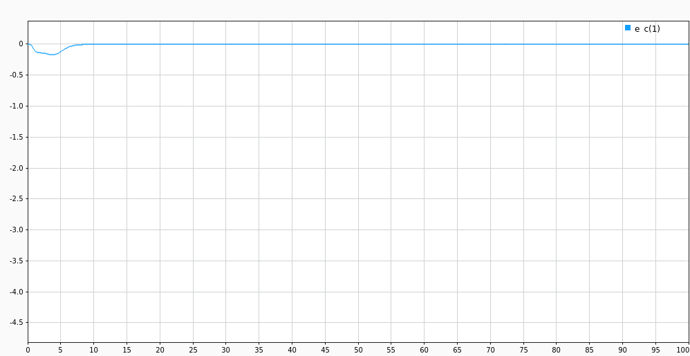
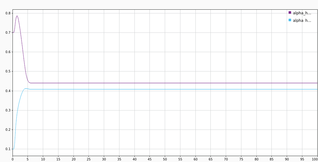
The tracking error is converging to 0 rapidly.
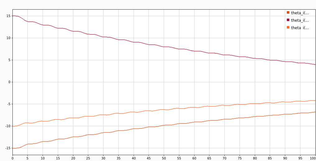
The individual parameter estimates are still converging to the plant values very slowly. But due to fast second level estimation of \(\alpha\) (as seen in next fig.), the system as a whole is converging down rapidly.
Result
Through qualitative analysis and simulations we have demonstrated the effectiveness of using multiple models for adaptive control, as introduced by the original paper [1].
References
[1] Z. Han and K. S. Narendra, “New Concepts in Adaptive Control Using Multiple Models,” in IEEE Transactions on Automatic Control, vol. 57, no. 1, pp. 78-89, Jan. 2012. doi: 10.1109/TAC.2011.2152470